Pipeline workflow

The following describes the steps that each observations launched by the pipeline takes.

Get archives and metadata

The pipeline uses psrdb.py to get the metadata of an observation including, the UTC start time, the pulsar PSRJ name, the project short code (PTA, RelBin, TPA or GC), the beam number and the centre frequency. This information is used to find the location of the archive files on OzSTAR:

/fred/oz005/timing/<pulsar_jname>/<UTC_start>/<beam_number>/<centre_frequency_MHz>/

These archives come out of the MeerKat pulsar backend (the Pulsar Timing User Supplied Equipment (PTUSE) Bailes et al. 2020) as individual eight second archive files. We use the psradd command (a psrchive script) to combine these archives into a single archive for further processing.

Calibrate

The delays are corrected with the dlyfix command (from the dylfix repo). Depending on the date of the observations, the polarisation is either already applied before being transferred to OzSTAR, or must be applied using a Jones matrix. The jones matrix must be applied using the pac -Q command (a psrchive script) for UHF band observations prior to approximately 18/08/2021 and L-band observations prior to approximately 10/04/2020. Observations after these dates only need to have their polarisation headers updated with the pac -XP command.

The data is also corrected for the Faraday rotation using the rotation measure (RM) and their dispersion measure (DM) if known, from a RM and DM list provided from the project configuration or the ATNF Pulsar Catalogue.

Clean

The archives are cleaned of RFI using the command clean_archive.py (a MeerGuard script). The cleaning is done by applying the following three “cleaners”:

rcvrstd: zaps out specified channels / subints / band edges, etc. Doesn’t do any thinking of its own, just zaps according to a fixed set of input parameters
surgical: uses the template to assess off-pulse windows and statistics to identify parts of the data which deviate due to RFI
bandwagon: zaps out the remaining portion of a channel / subint if the fraction of that subint/channel that has already been zapped is above a certain fraction

Decimation

The data are then decimated, reduced in resolution across any of the time, frequency and polarisation axes per the scientific needs of the project. This is done with the following psrchive command

pam --setnsub <nsub> --setnchn <nchan> -S <stokes_op>

The decimation products are specified via the config file, and that the products can be tuned specific to each pulsar. Common values for nsub are 1, 32 and 450. Common values for nchan are 1, 16 and 32.

Flux calibrate

The flux calibration is performed by the fluxcal.py command (a meerpipe script). It adjusts the archive units so they are in flux units by multiplying them by the expected RMS and dividing them by the observed RMS (\(C_F=\sigma_c/\sigma_\mathrm{obs}\)). The observed RMS is the median RMS of the off pulse values of the centre channels (1383-1400 MHz for LBAND and 795-805 MHz for UHF band). The expected RMS (\(\sigma_c/\)) is obtained from the following equation based on Equation 1 of Posselt et al. (2023):

\[\sigma_c = \frac{\mathrm{SEFD}+T_{\mathrm{sky}}}{ N_{\mathrm{ant}} \sqrt{2 \times \Delta \nu_{\mathrm{bw}} N_{\mathrm{ch}}^{-1} \times t_{\mathrm{obs}} N_{\mathrm{bin}}^{-1} }}\]

Where \(\mathrm{SEFD}\) is the known system equivalent flux density for a single dish, \(T_{\mathrm{sky}}\) is the expected sky temperature, \(N_{\mathrm{ant}}\) is the number of antenna, \(\nu_{\mathrm{BW}}\) is the frequency bandwidth, \(N_{\mathrm{chan}}\) is the number of frequency channels, \(t_{\mathrm{obs}}\) is the length of the observation and \(N_{\mathrm{bin}}\) is the number of phase bins in the pulse profile.

For LBAND the \(T_{\mathrm{sky}}\) map is obtained from the HIPASS ‘point-source’ continuum map at 1.4 GHz described in Calabretta et al. (2014) which has been altered by the method described in Posselt et al. (2023) to be comparable with MeerKAT’s smaller beam.

Create ToAs and residuals

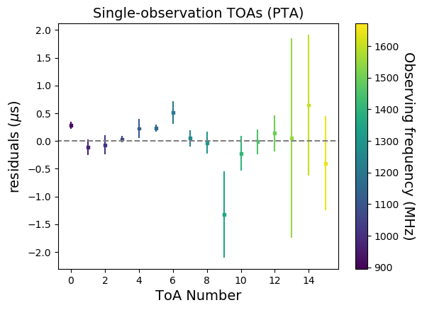
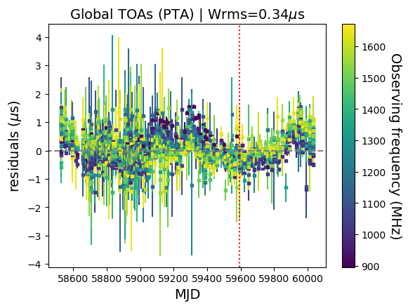
The pulse ToAs are calculated from each of the decimated data products using tempo2. Each project has their own templates and ephemerides the resulting ToAs and residuals may vary. A single ‘representative’ set of ToAs are also calculated; these are then used to produce residual plots both the ‘local’ ToAs specific to the observation being processed, as well as ‘global’ plots showing the performance of the timing model over all data recorded for the pulsar. These residuals are then plotting using the matplotlib software package to show the ephemerides as they are, without any additional fitting. Below is an example of J1909-3744’s single observation ‘local’ residuals:

single_residuals

And here is a plot showing ‘global’ residuals:

global_residuals

Make images

Also displayed for each observation are pre- and post-cleaned plots of time vs. phase, frequency vs. phase, flux vs. phase and stokes vs. phase. The following sub sections will show examples of these plots for J1240-4124

Stokes I Pulse profile

This plot is generated with the command:

psrplot -p flux -jFTDp -jC                -g 1024x768 -c above:l= -c above:c="Stokes I Profile"     {file}

Here is and example of the pre-cleaned plot:

and here is and example of the post-cleaned plot:

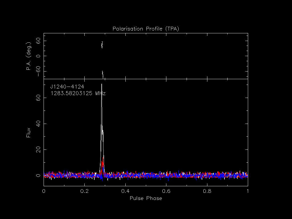
Polarisation profile

This plot is generated with the command:

psrplot -p Scyl -jFTD  -jC                -g 1024x768 -c above:l= -c above:c="Polarisation Profile" {file}

Here is and example of the post-cleaned plot:

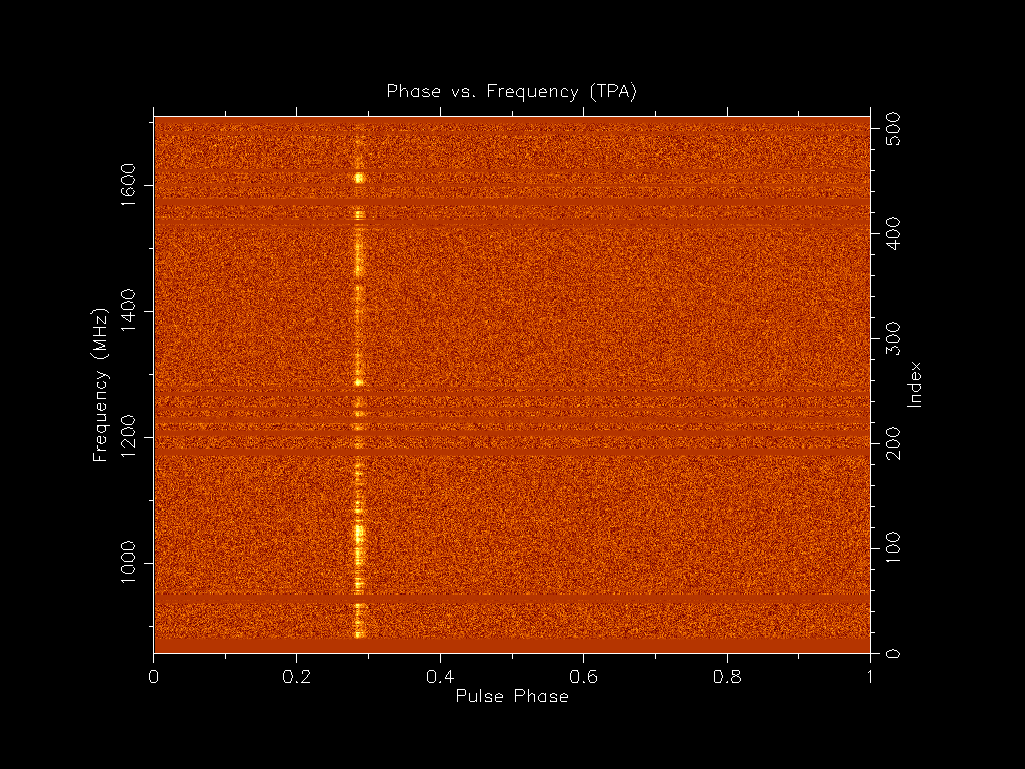
Phase vs. frequency

This plot is generated with the command:

psrplot -p freq -jTDp  -jC                -g 1024x768 -c above:l= -c above:c="Phase vs. Frequency"  {file}

Here is and example of the pre-cleaned plot:

raw_freq_phase

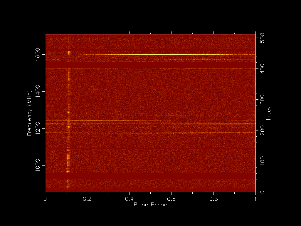
and here is and example of the post-cleaned plot:

clean_freq_phase

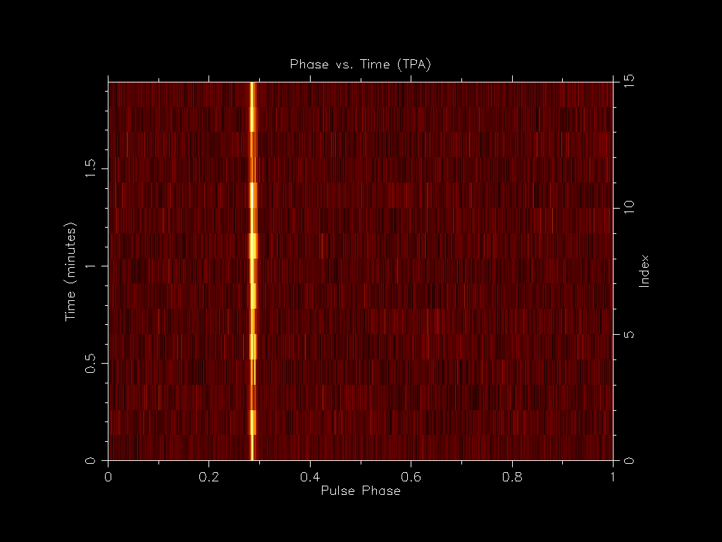
Phase vs. time

This plot is generated with the command:

psrplot -p time -jFDp  -jC                -g 1024x768 -c above:l= -c above:c="Phase vs. Time"       {file}

Here is and example of the pre-cleaned plot:

raw_time_phase

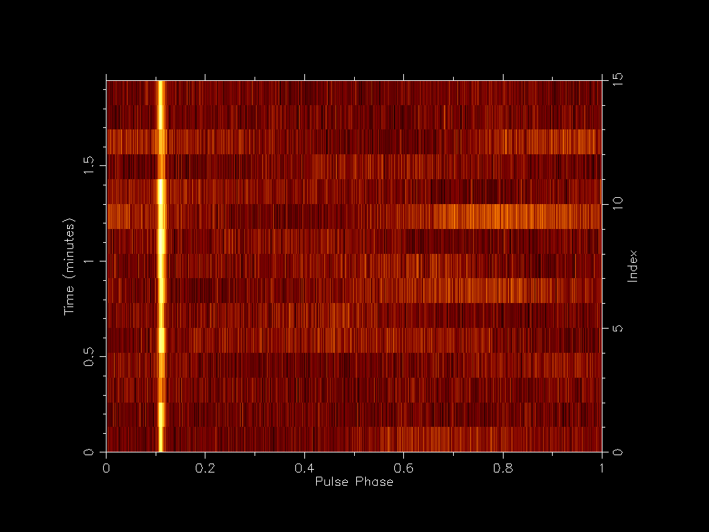
and here is and example of the post-cleaned plot:

clean_time_phase

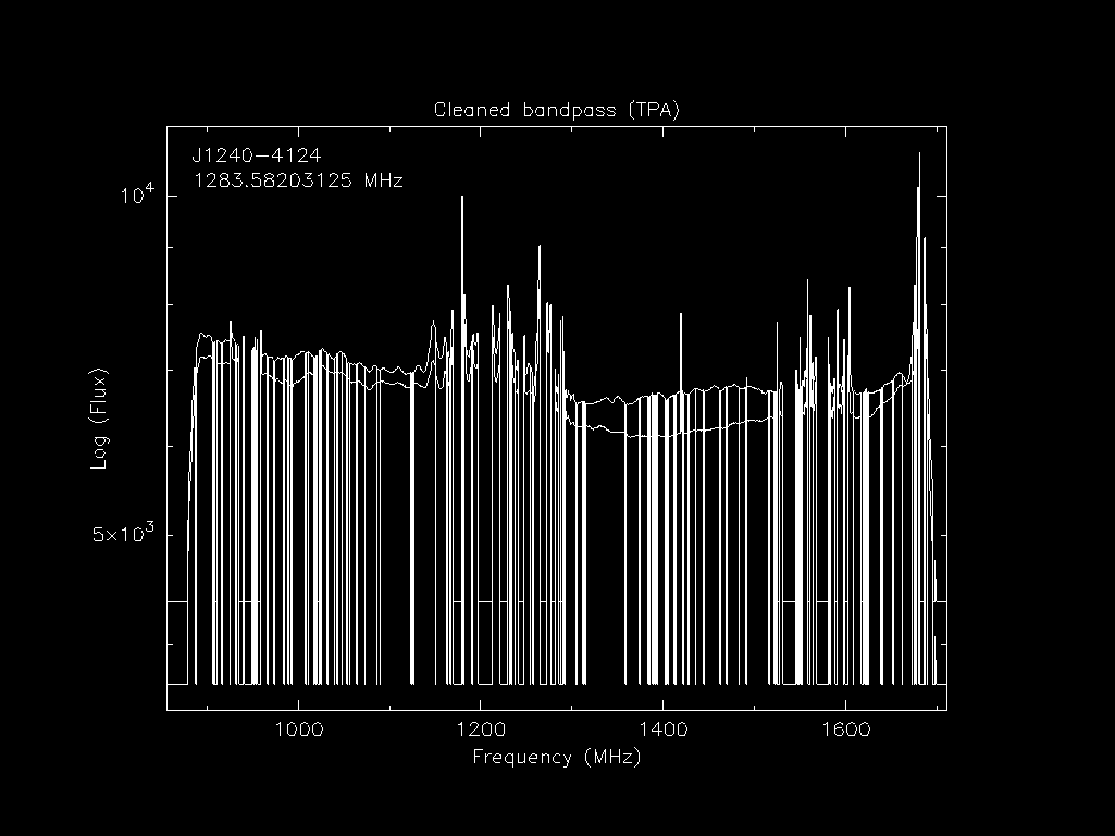
Bandpass

This plot is generated with the command:

psrplot -p b -x -jT -lpol=0,1 -O -c log=1 -g 1024x768 -c above:l= -c above:c="Cleaned bandpass"     {file}

Here is and example of the pre-cleaned plot:

raw_bandpass

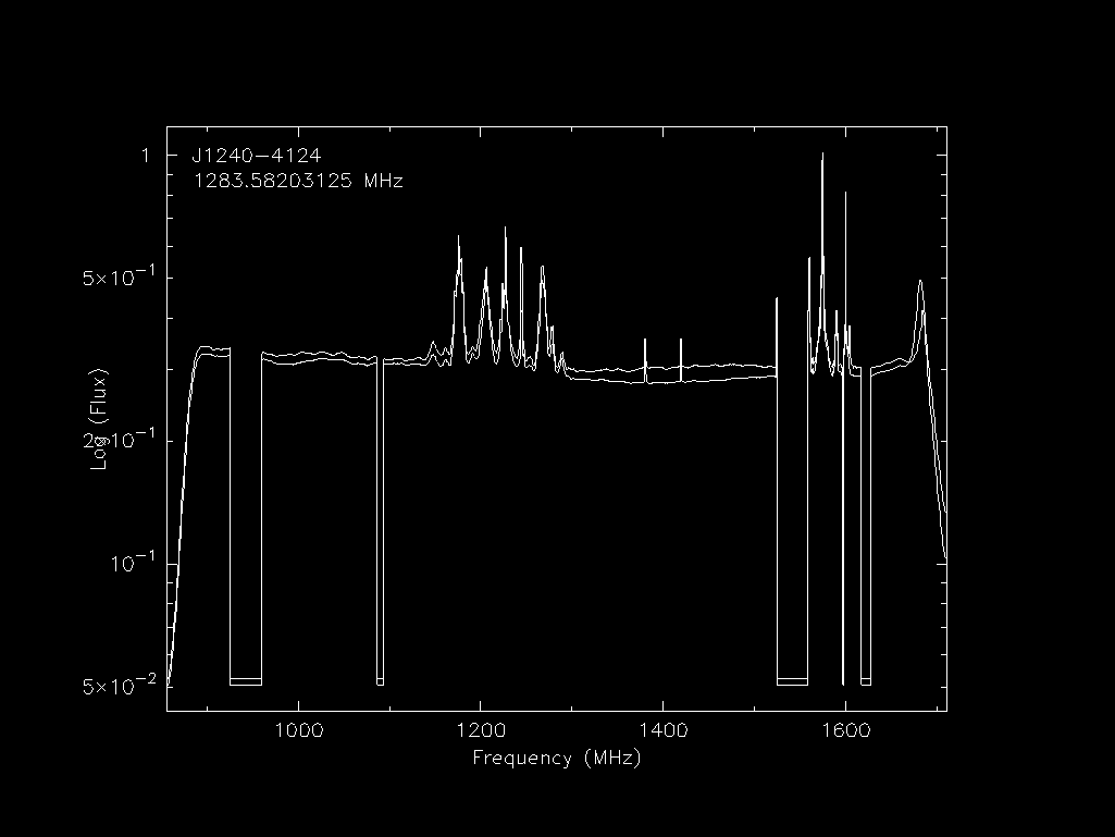
and here is and example of the post-cleaned plot:

clean_bandpass

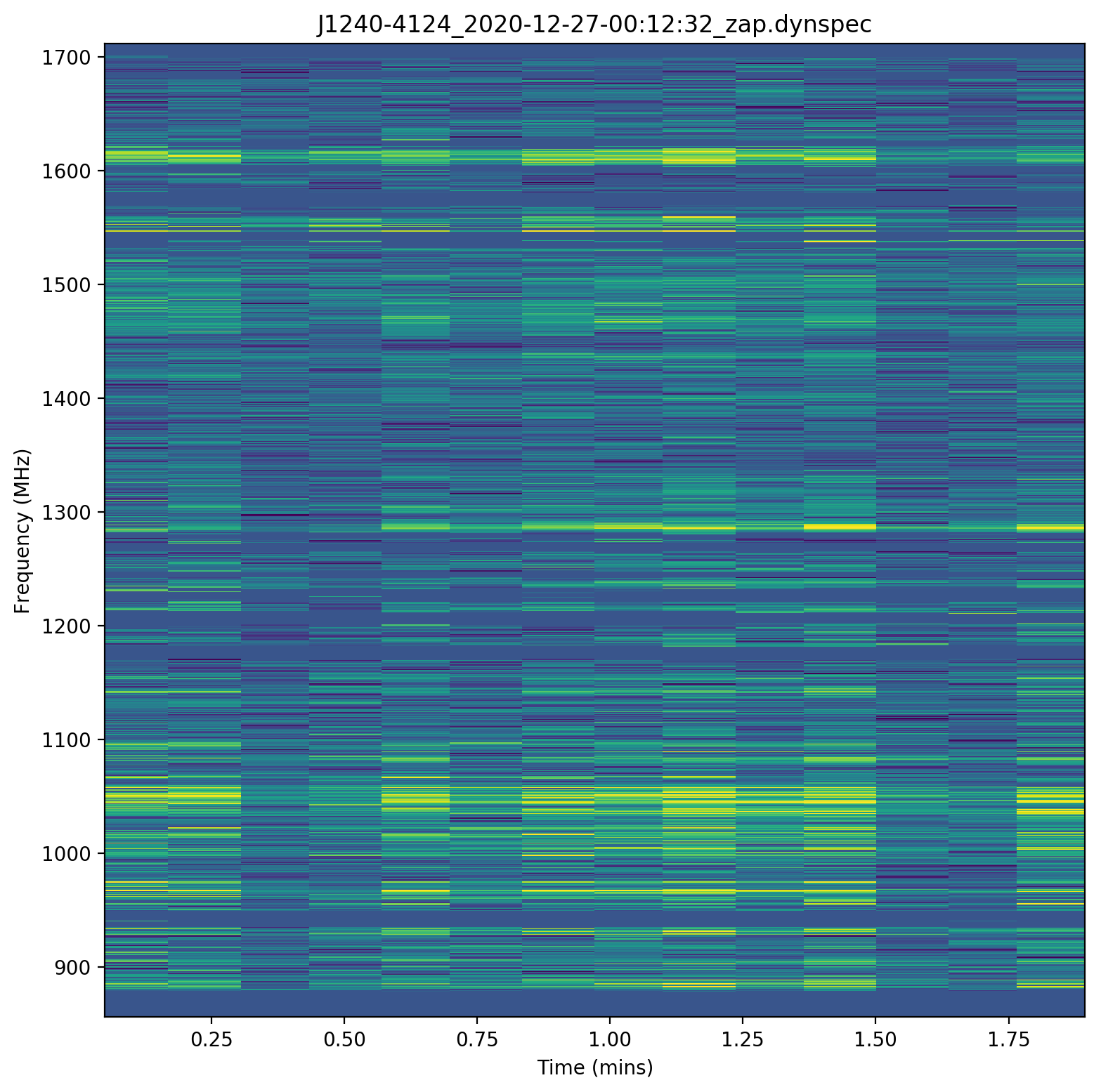
Dynamic spectra

The dynamic spectra are produced by the scintools software package.

Here is and example of the pre-cleaned plot:

raw_dynamic_spec

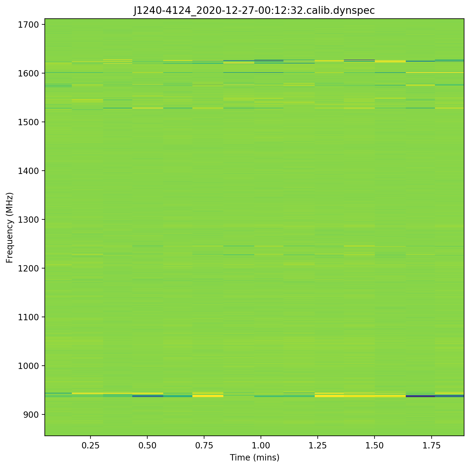
and here is and example of the post-cleaned plot:

clean_dynamic_spec

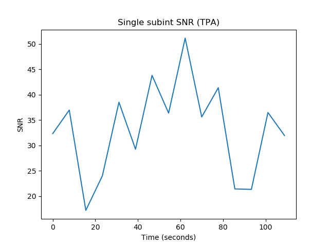
Signal-to-noise ratio

The following signal-to-noise plots are created with matplotlib using the meerpipe scripts

Here is and example of the pre-cleaned plot:

raw_snr

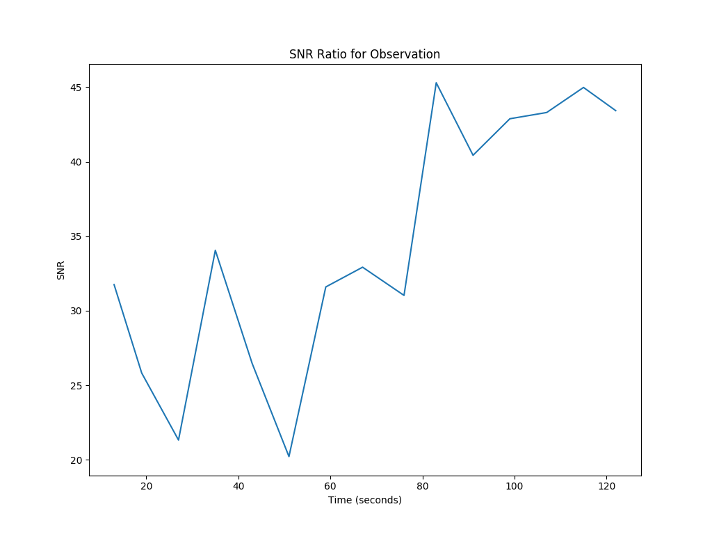
and here is and example of the post-cleaned plot:

clean_snr

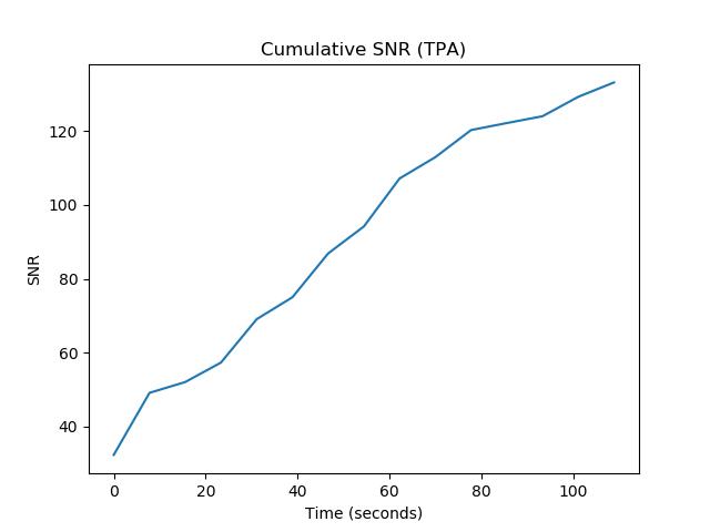
and here is an example of the post-cleaned plot that shows cumulative S/N instead of instantaneous:

cumlative_snr

Upload

These images, the total S/N, flux density, zapped-RFI fraction are uploaded to the portal via psrdb.py